Discrete phase space

Contents:

• The discrete Fourier transform
• Translations in phase space
  • Horizontal translations
  • Vertical translations

Some very rough notes on discrete phase space, specifically the simplest case of 2 position and 2 momentum states forming a 2x2 grid like this:

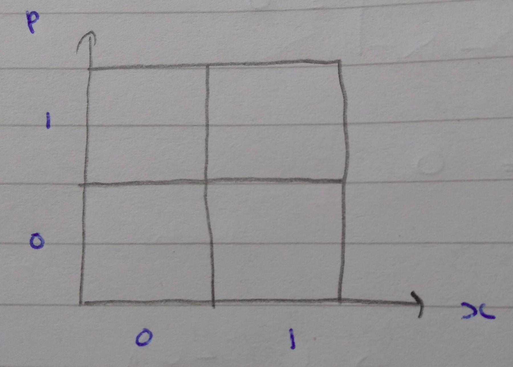
(I’m mostly interested in this for its connections to the Spekkens toy model, which uses a similar 2x2 grid of states.)

I want to find the discrete Wigner function on this 2x2 phase space. This is defined by analogy to the continuous one (notes on that here). For a start, we’re going to want discrete analogues of:

and

For a 2x2 system this is just the four equations

Or, in picture form:

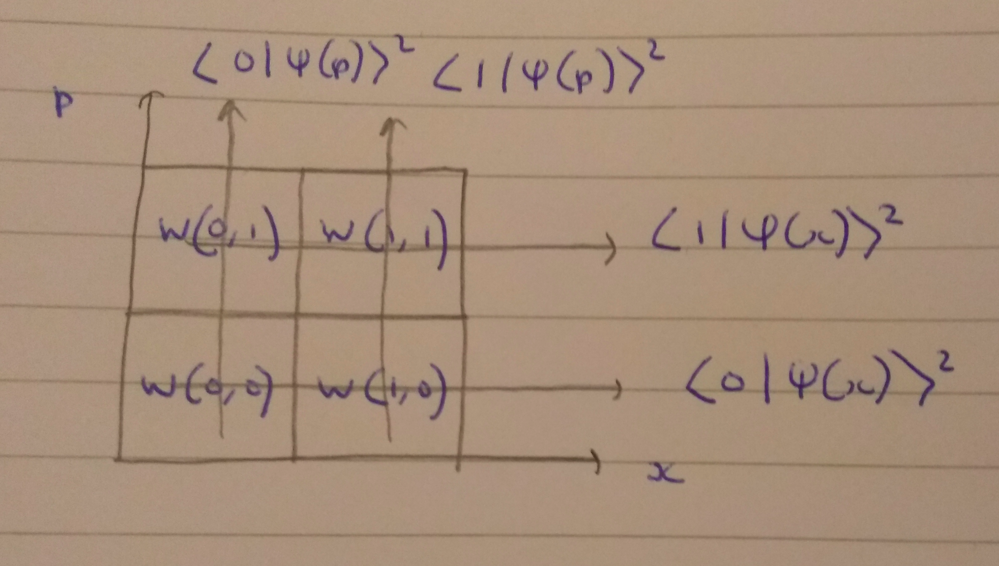
The quantities \(\langle 0 \vert \psi(x) \rangle ^2\) etc are what we actually measure, and we want to use these to infer the Wigner function \(W(x,p)\). There’s not enough information to do this uniquely, yet - we would also need to specify how the sums along the diagonals relate to measurements. I’ll talk about that later.

The continuous version of this is called the inverse Radon transform, which tranforms a function over lines to a function on points. It’s used in medical tomography to e.g. reconstruct an image of the density of the brain by taking X-ray measurements, which give a line integral of the density along the X-ray path. (The quantum state equivalent is called quantum tomography by analogy).

The discrete Fourier transform

Position and momentum are Fourier pairs, so we’re going to want to Fourier transform between them. The discrete Fourier transform for two points is pretty simple (see e.g. here): for \(\vert\psi\rangle = a\vert z_+\rangle + b\vert z_-\rangle\), the Fourier transform is \(\vert\tilde{\psi}\rangle = F\vert\psi\rangle\), where \(F\) is the matrix

So, in components,

i.e.

So the 2 point DFT transforms between the \(z\) component representation and the \(x\) component one.

Translations in phase space

(For this section I’ll mostly be following Picturing Qubits in Phase Space by Wootters.)

The 2x2 phase space is normally used for qubit states. In this case it’s usual to take the horizontal axis as the \(z\) component of spin, and the vertical axis as the \(x\) component. So I’ll relabel the axes in this way:

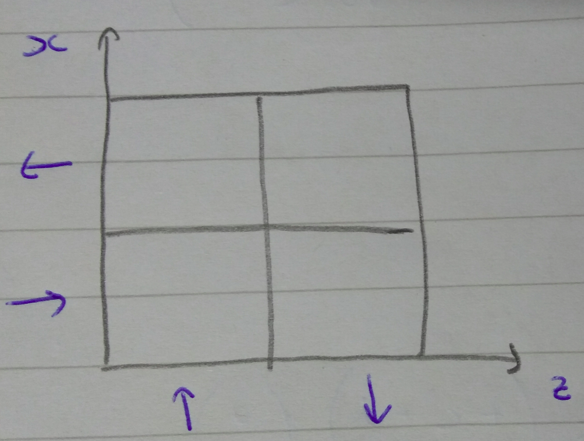
We’ll define horizontal and vertical translations on phase space in terms of their action on the state \(\vert\psi\rangle\).

Horizontal translations

Horizontal translations \(H\) rearrange phase space cells like this:

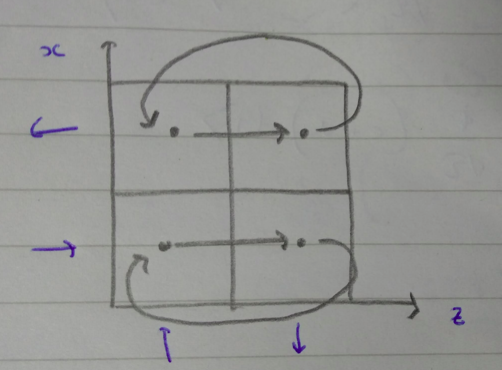
This swaps the two columns, so we should expect \(\vert z_+\rangle\) and \(\vert z_-\rangle\) states to be interchanged. This can be achieved with the operator

This is the Pauli matrix \(\sigma_x\), which acts on \(\vert z_+ \rangle\), \(\vert z_- \rangle\) as follows:

So the two states are interchanged as expected.

For \(\vert x_+ \rangle\) and \(\vert x_- \rangle\), we have:

So \(\vert x_+\rangle\) is unchanged, and \(\vert x_-\rangle\) is reversed.

(Not quite sure why reversing \(\vert x_-\rangle\) is OK. Maybe because normal QM takes place on a projective space, where \(\lambda\vert\psi\rangle\) and \(\vert\psi\rangle\) represent the same state? Maybe the same is true in this toy model.)

Vertical translations

Similarly, vertical translations \(V\) rearrange phase space like this:

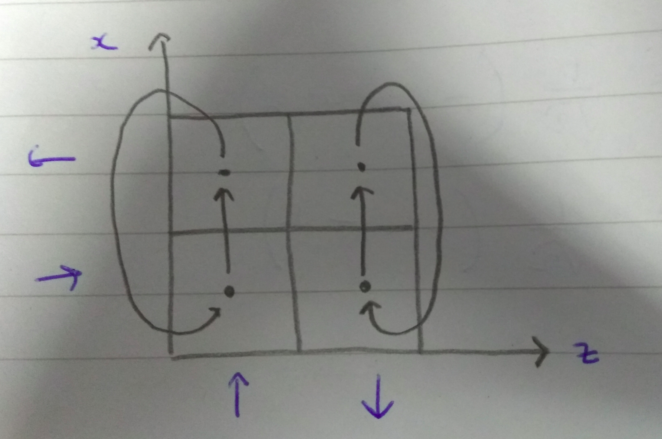
This time the states \(\vert x_+\rangle\) and \(\vert x_-\rangle\) are interchanged. This can be done with the operator

This is the Pauli matrix \(\sigma_z\). It acts on \(\vert x_+ \rangle\) and \(\vert x_- \rangle\) as:

So the components are swapped as expected. For \(\vert z_+ \rangle\), \(\vert z_- \rangle\) we have

So \(\vert z_+\rangle\) is unchanged and \(\vert z_-\rangle\) is reversed.