The Wigner function

Jul 17, 2018

First I wondered if going back to the original paper would be helpful. Turns out no. Wigner states that ‘one may build the following expression’, writes down the formula, and then adds this helpful footnote: ⊕ I searched a bit, and it looks like Szilard may have never been involved - Wigner just wanted to boost Szilard’s career when he got out of Germany in the 30s. Haven’t found the original source yet, but see e.g. here. The reference is to ‘R. F. O’Connell (private communication)’.

‘Me and my mate thought of it once, but we won’t tell you where or how.’ Thanks, Wigner!

So I had to look elsewhere. One of my starting points was these two blog posts about the Wigner function by Jess Riedel, a physicist who also got annoyed by the usual way it’s introduced. He makes the point vividly by introducing the ‘Jigner function’ \(J(x,p) = \vert\psi(x)\vert^2\vert\psi(p)\vert^2\), a pointless function he just made up. \(J(x,p)\) also reproduces the position and momentum distribution, but is otherwise not very illuminating. So what’s special about the Wigner function?

I’ve ended up exploring along a somewhat different path, but I’ll get to Riedel’s version at the end. This page is supposed to be notes-in-progress rather than a finished post - I’m still in the process of doing this and you will notice a lot of To dos and To adds in this post.

Time-frequency analysis and musical notation

The first interesting thing I learnt was that the Wigner function is also used in classical physics, in the field of time-frequency analysis. Time and frequency are Fourier pairs in classical physics in the same way that position and momentum are in quantum physics. This means you can’t measure both of them precisely at the same time: a precisely localised position measurement will map to a fully spread out infinite sinusoid, and vice versa. So trying to plot time against frequency precisely for a signal is always going to be something of a bodge.

Terence Tao teaches a course on time-frequency harmonic analysis, and in the introduction he points out that actually people do try to plot frequency and time at once. Despite being slightly fake mathematically, it has a long history and is very useful:

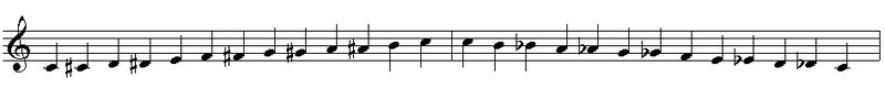
I had never thought about this before! Musical notation is just time along the x axis and frequency up the y axis:

We would normally say that that first middle C has a frequency of 256 Hz, and strictly that only applies if you play it for all of time, to get an infinite sinusoid. In reality, though, all you want is for the waveform to be reasonably periodic at 256 Hz for the half a second or so that the note is supposed to last. The musical score does a good job of summarising the information you actually want, and that you won’t get from just looking at a position or frequency plot on its own.

I found a nice description of this in this 1967 paper by de Bruijn:

For example, if \(f\) represents a piece of music, then the composer does not produce \(f\) itself; he does not even define it. He may try to prescribe the exact frequency and the exact time interval of a note (although the uncertainty principle says that he can never be completely successful in this effort), but he does not try to prescribe the phase. The composer does not deal with \(f\); it is only the gramophone company which produces and sells an \(f\). On the other hand, the composer certainly does not want to describe the Fourier transform. This Fourier transform is very useful for solving mathematical and physical problems, but it gives an absolutely unreadable picture of the given piece of music.

What the composer really does, or thinks he does, or should think he does, is something entirely different from describing either \(f\) or \(\mathcal{F}f\). Instead, he constructs a function of two variables. The variables are the time and the frequency, the function describes the intensity of the sound. He describes the function by a complicated set of dots on score paper. His way of describing time is slightly different from what a mathematician would do, but certainly vertical lines denote constant time, and horizontal lines denote constant frequency.

The short time Fourier transform

There’s lots of theory in signal processing on different ways to produce functions that are something like a mathematical version of the composer’s score, functions that show how the signal behaves in both frequency and time. The simplest option is the short term Fourier transform. ⊕ This sort of spectrogram got some unexpected publicity in mid-2018 while I was researching this! You start in the time domain, keep the signal for a small chunk (‘window’) of time and set the rest to zero, and calculate the Fourier transform of that to get a local frequency:

\[\begin{equation} STFT (\tau, \omega) = \int^\infty_{-\infty} \psi(t) w(t - \tau) e^{-i\omega t} dt \end{equation}\]

where in the simplest case the ‘window function’ \(w\) is just a boxcar function that’s \(1\) for a small chunk of the domain and \(0\) everywhere else.

For the musical example above, if your window covers the duration of the middle C you’ll pick up the 256 Hz. Then you move your window along a bit in time to pick up some different frequencies:

Sketch of the basic idea of a short time Fourier series. The original time series is at the top, and short windows of it are mapped to frequency curves. Think of each frequency curve as sticking up out of the page.

There’s an underlying symmetry in the Fourier transform, so that you could instead start in the frequency domain and take short windows of that, and transform to the time domain. This would be a pretty stupid choice in music, I think, because the signals we want to listen to tend to have spread-out, periodic behaviour in time rather than frequency. (On the other hand there are some important features in music that are narrow in time but wide in frequency, like the ‘attack’ at the start of a bowed string note, where it might be better?) But really it’s a trade off… you either end up with good time resolution or good frequency resolution.

Other window functions

To do better than this, you can make a cleverer choice of window function. Using a Gaussian window turns out to be the best compromise between resolution in time and resolution in frequency. This is called the Gabor transform.

The ‘symmetric’ short time Fourier transform

This doesn’t seem to be a common thing to do with the STFT, but it will be useful for comparing with the Wigner function. In the ‘normal’ STFT, we keep the function \(\psi\) static and move the window function \(w\) along. It would also be possible to move to the frame midway between them, so that the function is going ‘backwards’ at the same speed the window is going ‘forwards’. We can do this by substituting in \(T = t - \frac{\tau}{2}\), to get

\[\begin{equation} SSTFT (\tau, \omega) = \int^\infty_{-\infty} \psi\left(T + \frac{\tau}{2}\right) w\left(T - \frac{\tau}{2}\right) e^{-i\omega t} dt \end{equation}\]

where \(SSTFT\) is my clunky notation for the ‘symmetric’ short time Fourier transform.

Back to the Wigner function

To compare this to the Wigner function, we can first follow Riedel in making the substitution \(y = \frac{\Delta x}{2}\), to make \(W(x,p)\) look more like a normal Fourier transform of something:

\[\begin{equation} W(x, p) = \frac{1}{2\pi} \int^\infty_{\infty} \psi^*\left(x + \frac{\Delta x}{2}\right) \psi\left(x - \frac{\Delta x}{2}\right) e^{-ipy} dy. \end{equation}\]

Now we can see that in these coordinates the Wigner function is very similar to the symmetric STFT. We’re back in position/momentum space instead of time/frequency (the Wigner function is used in time/frequency space as well, but I want to get back to its use in quantum physics now). But the main difference is that the window functon is just \(\psi^*\)! We’re doing a sort of autocorrelation, rather that bringing in a new outside function to use as the window. ⊕ OK, there’s also a factor of \(2\pi\) difference. Not sure if that’s different Fourier transform conventions, or the \(2\pi\) gets folded into \(w\) in the STFT, or what. I can’t be bothered to track it down.

This is very similar to the viewpoint Riedel ended up with in his first post… he writes the \(W(x,p)\) in terms of the density matrix (which is pretty much just an autocorrelation anyway) and then shows that it’s the Fourier transform of the density matrix in rotated coordinates. This might be better for understanding what the entries mean. But I find that situating the Wigner function within the class of other phase space transforms is also helpful for my understanding.

Wigner function as expectation value of the parity operator

Haven’t looked into this much yet, but possibly related: it’s apparently also possible to consider the Wigner function as the expectation value of the parity operator that reflects points in phase space. Or, as the paper puts it (it uses \(f\) instead of \(W\)):

Alternatively, \(f(r, p)\) is proportional to the overlap of \(f\) with its mirror image about \(r,p\), which is clearly a measure of how much \(f\) is “centered” about \(r,p\).

To do: actually read the paper!

Wigner function from phase space symmetries

To do: expand this section

This paper by Wootters explains that actually the Wigner function has a more elegant property than just reproducing the position and momentum distributions, which goes something like this: you can integrate along any line in phase space and get a similar marginal distribution, but for an observable that’s some linear combination of position and momentum. This seems to be the neatest way of answering Riedel’s question of why we use the Wigner function specifically, and not one of the many other functions that only reproduce the position and momentum marginals.

It makes sense that you’d want some property like that if you want the Wigner function to respect Galilean invariance, and still get something that makes sense if you transform your position and velocity coordinates.

The exact statement is a little more involved than my summary above, and works over an infinite strip of phase space rather than just a line. Quoting from Wootters:

Let the state of a particle in one dimension be given by the Wigner function \(W\). Consider the integral of \(W\) over the infinite strip of phase space bounded by the two parallel lines \(aq + bp = c_1\), and \(aq + bp = c_2\). (Here \(a, b, c_1,\) and \(c_2\) are arbitrary real numbers.) This integral is equal to the probability that the observable \(a\hat{q} + b\hat{p}\) for this particle will be found to have a value between \(c_1\) and \(c_2\).

Wigner function as ‘convolutionary mean’

Jess Riedel’s second post takes a different path to understanding the Wigner function, explaining that it’s the ‘convolutionary mean’ of two other distributions that quantum optics people like for some reason, the Glauber-Sudarshan \(P\) distribution and the Husimi \(Q\) distribution. (‘Convolutionary mean’ is a useful term Riedel makes up - it means that \(W\) is ‘halfway’ between \(P\) and \(Q\) in the sense that \(P * g = W\) and \(Q = W * g\) where \(g\) is some Gaussian that’s explained in the post).

To do: learn what the hell these distributions are. Start by reading the blog post properly!

This looks somewhat similar to the way it was introduced in Ville’s original paper. (Ville was the person who independently introduced the Wigner function to signal processing, where it is often known as the Wigner-Ville distribution.) ⊕ Ville was not a big name like Wigner: he worked at the telecommunications lab at the Société Alsacienne de Constructions Mécaniques, rather than a fancy university, and he published in an obscure journal called Câbles et Transmissions. So nobody really read his paper. Ville’s paper also looks well worth reading properly - it gives a lot more setup that Wigner did, and makes connections with lots of important stuff to do with operator ordering and the Wigner-Weyl transform.

Ville tries to write down a characteristic function for the distribution on time-frequency space, and runs into operator-ordering issues. He looks at the two most obvious choices of ordering given the situation (which I think may correspond to normal and anti-normal ordering), and rules them out for symmetry reasons. He then finds that a ‘halfway’ option of taking the geometric mean does work - I think this may correspond to the Weyl ordering.

To do: go through the details, check that these do correspond to normal, anti-normal, and Weyl ordering. Also, is there a link between his ‘two most obvious choices’ and the \(P\) and \(Q\) distributions?