Qubit phase space cheat sheet
Contents:
Like my other qubit cheat sheet, but specifically for phase-space-related things.
Phase point operators
These can be used to construct the Wigner function \(W\) given a density matrix \(\rho\). They satisfy
\[\begin{equation} W_{ij} (\rho) = \frac{1}{2} \text{Tr}(\rho A_{ij}) \end{equation}\]See Wootters 1987 for more on these.
\[\begin{equation} A_{00} = \frac{1}{2}\left( \begin{array}{cc} 2 && 1-i \\ 1+i && 0 \\ \end{array} \right) \end{equation}\] \[\begin{equation} A_{01} = \frac{1}{2}\left( \begin{array}{cc} 2 && -1+i \\ -1-i && 0 \\ \end{array} \right) \end{equation}\] \[\begin{equation} A_{10} = \frac{1}{2}\left( \begin{array}{cc} 0 && 1+i \\ 1-i && 2 \\ \end{array} \right) \end{equation}\] \[\begin{equation} A_{11} = \frac{1}{2}\left( \begin{array}{cc} 0 && -1-i \\ -1+i && 2 \\ \end{array} \right) \end{equation}\]Wigner function for a qubit
Now apply this to a general qubit of the form
\[\begin{equation} |\psi\rangle = \left( \begin{array}{c} \cos (\frac{\theta}{2}) \\ e^{i\phi}\sin (\frac{\theta}{2}) \\ \end{array} \right) \end{equation}\]Find that
\[\begin{equation} W_{00} = \frac{1}{4}\left[1 + \cos\theta + \sin\theta(\cos\phi + \sin\phi) \right] \end{equation}\] \[\begin{equation} W_{01} = \frac{1}{4}\left[1 + \cos\theta - \sin\theta(\cos\phi + \sin\phi) \right] \end{equation}\] \[\begin{equation} W_{10} = \frac{1}{4}\left[1 - \cos\theta + \sin\theta(\cos\phi - \sin\phi) \right] \end{equation}\] \[\begin{equation} W_{11} = \frac{1}{4}\left[1 - \cos\theta - \sin\theta(\cos\phi - \sin\phi) \right] \end{equation}\]It’s common to write these in a 2x2 box:
\[\begin{equation} W = \left[ \begin{array}{c|c} W_{01} & W_{11} \\ \hline W_{00} & W_{10} \\ \end{array} \right] \end{equation}\]Marginal probabilities
These are the probabilities that the rows, columns and diagonals of the Wigner function add up to when written in the box form above. Maybe an image would help:
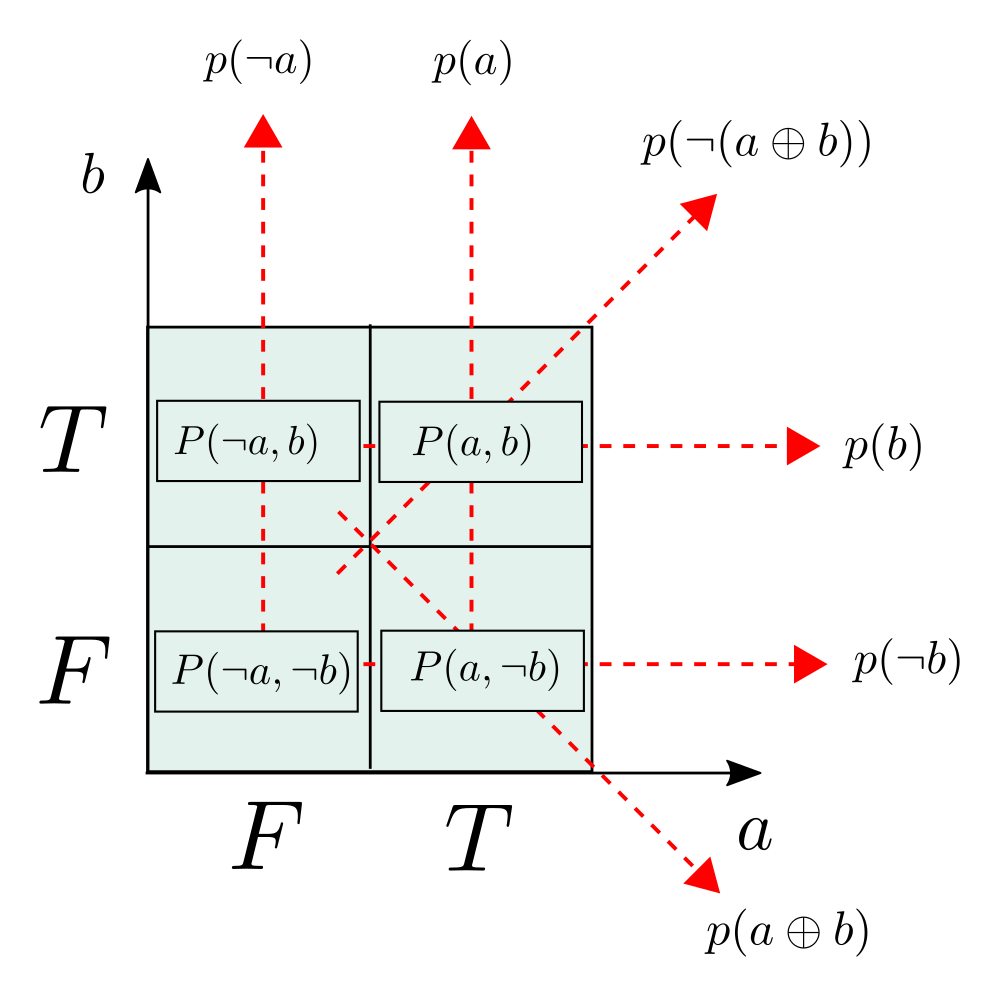
I’m using \(a\) and \(b\) for the axes in that image to fit in with what I needed for a blog post. It would be more normal to call them \(x\) and \(z\) respectively, but I can’t be bothered to redraw the figure.
These satisfy the formula
\[\begin{equation} p_i = \frac{1}{2} - \frac{1}{2}\langle\psi | \sigma_i | \psi \rangle . \end{equation}\]where \(p_z = p(a)\), \(p_x = p(b)\), \(p_y = p(a\oplus b)\). For a general qubit these are:
\[\begin{equation} p_z = \frac{1}{2} - \frac{1}{2}\cos\theta. \end{equation}\] \[\begin{equation} p_x = \frac{1}{2} - \frac{1}{2}\sin\theta\cos\phi. \end{equation}\] \[\begin{equation} p_y = \frac{1}{2} - \frac{1}{2}\sin\theta\sin\phi. \end{equation}\]Examples
Here are some examples of Wigner functions.
Pauli matrix eigenstates
+1 eigenstate of \(\sigma_z\):
\[\begin{equation} \left[ \begin{array}{c|c} \frac{1}{2} & 0 \\ \hline \frac{1}{2} & 0 \\ \end{array} \right] \end{equation}\]-1 eigenstate of \(\sigma_z\):
\[\begin{equation} \left[ \begin{array}{c|c} 0 & \frac{1}{2} \\ \hline 0 & \frac{1}{2} \\ \end{array} \right] \end{equation}\]+1 eigenstate of \(\sigma_x\):
\[\begin{equation} \left[ \begin{array}{c|c} 0 & 0 \\ \hline \frac{1}{2} & \frac{1}{2} \\ \end{array} \right] \end{equation}\]-1 eigenstate of \(\sigma_x\):
\[\begin{equation} \left[ \begin{array}{c|c} \frac{1}{2} & \frac{1}{2} \\ \hline 0 & 0 \\ \end{array} \right] \end{equation}\]+1 eigenstate of \(\sigma_y\):
\[\begin{equation} \left[ \begin{array}{c|c} 0 & \frac{1}{2} \\ \hline \frac{1}{2} & 0 \\ \end{array} \right] \end{equation}\]-1 eigenstate of \(\sigma_y\):
\[\begin{equation} \left[ \begin{array}{c|c} \frac{1}{2} & 0 \\ \hline 0 & \frac{1}{2} \\ \end{array} \right] \end{equation}\]Examples with negative probabilities
Note that the marginal probabilities are still always positive.
+1 eigenstate of \(\frac{1}{\sqrt{2}} (\sigma_z + \sigma_x)\):
\[\begin{equation} \left[ \begin{array}{c|c} \frac{1}{4} & \frac{1 - \sqrt{2}}{4} \\ \hline \frac{1 + \sqrt{2}}{4} & \frac{1}{4} \\ \end{array} \right] \end{equation}\]-1 eigenstate of \(\frac{1}{\sqrt{3}} (\sigma_z + \sigma_x + \sigma_y)\):
\[\begin{equation} \left[ \begin{array}{c|c} \frac{1}{4}\left(1+ \frac{1}{\sqrt{3}}\right) & \frac{1}{4}\left(1+ \frac{1}{\sqrt{3}}\right) \\ \hline \frac{1}{4}\left(1 - \sqrt{3}\right) & \frac{1}{4}\left(1+ \frac{1}{\sqrt{3}}\right) \\ \end{array} \right] \end{equation}\]The bottom left value is the most negative possible for a qubit.